
Python · numba · scipy · FunctionalScale on GitHub
Overview
Classical GARCH treats a single number, the daily variance, as the thing worth modelling. Intraday data gives you a full curve instead, volatility has a shape across the trading day, not just a level. This project, developed jointly with André Lucas and Yicong Lin, treats intraday log-return paths as functions \(y_t(u)\) over the trading day \(u \in [0,1]\), and extends the GARCH recursion from a scalar update to an operator update over the whole curve, so a shock at any point in the day can feed into the entire upcoming volatility surface rather than a single end-of-day number. Where the Functional Scale Volatility Estimation project focuses on getting a single static functional GARCH(1,1) recursion estimated correctly, this project extends the same Bernstein-basis idea to a genuinely time-varying, score-driven model, and is the computational engine behind the fast, scalable estimation methodology shared across this collaboration.
Theoretical Integration
The theory here draws on two papers. Cerovecki, Francq, Hörmann & Zakoïan (2018) supply the functional GARCH(1,1) baseline and its quasi-likelihood estimation theory, see the companion project page for the full exposition of that model in the notation used here. Lin & Lucas (2025, "Functional Location-Scale Models with Robust Observation-Driven Dynamics", Tinbergen Institute Discussion Paper TI 2025-027/III) supply the score-driven updating mechanism that this project's GAS-GARCH model implements. Their paper covers a much more general setting, joint location and scale dynamics over an arbitrary functional dimension, on sparsely observed data. This codebase implements the specific corner of that framework needed for intraday volatility, scale dynamics only, on a regular intraday grid, harmonised with the notation of the previous page.
As before, we work in \(H = L^2([0,1])\) with the functional scale model \[y_t(u) = \sigma_t(u)\,\eta_t(u), \qquad \sigma_t^2 = \delta + \sum_{i=1}^q \alpha_i(y_{t-i}^2) + \sum_{j=1}^p \beta_j(\sigma_{t-j}^2),\] the functional GARCH(1,1) model from the previous page. Projecting \(\delta\), \(\alpha_i\) and \(\beta_j\) onto a finite basis turns this recursion into a recursion for the basis-coefficient vector \(\gamma_i\) itself, \[\gamma_{i+1} = \omega + \bar{B}\,\gamma_i + A \int \varphi(s)\,y_i^2(s)\,ds,\] an update driven purely by the previous day's squared-return curve. The GAS extension changes only the driving term. Instead of feeding in the raw squared-return projection, it feeds in the score of a fat-tailed log-likelihood, so the size of today's update to \(\gamma_i\) depends on how surprising today's observation was, not just on its magnitude.
Estimation Procedure
The GAS recursion for the B-spline coefficient vector \(\gamma_i\) is \[\gamma_{i+1} = \omega + A\,s_i + B\,\gamma_i,\] where \(s_i\) is the scaled score of the model's log-likelihood at day \(i\), \(\omega\) is a constant, \(B\) governs persistence, and \(A\) governs the sensitivity of the update to new information. Returns are modelled as a zero-mean Student-\(t\) process rather than Gaussian, so a day with an unusually large or noisy intraday return is automatically downweighted when the score is computed. This is the same robustness property that makes score-driven models attractive in the classical, finite-dimensional case, carried over to the functional setting. The covariance across intraday grid points is itself modelled as a Student-\(t\) Ornstein–Uhlenbeck process, so grid points close together in intraday time are allowed to be more strongly correlated than distant ones. The static parameters \(\omega,A,B\), together with the Student-\(t\) degrees of freedom and the OU decay parameter, are estimated by maximising the resulting average log-likelihood over the sample. Lin & Lucas establish stationarity, ergodicity, filter invertibility, strong consistency and asymptotic normality of this estimator under regularity conditions analogous to those used for the functional GARCH QMLE on the previous page.
The funcgarch package's GAS-GARCH implementation is this scale-only case. It replaces the
Bernstein basis with a general B-spline basis, more flexible for smoothing a curve that is expected to drift
over the sample, and uses the Ornstein–Uhlenbeck kernel for the Student-\(t\) covariance across the
intraday grid. The B-spline coefficient vector plays the role of \(\gamma_i\) above, and its
score-driven update lets the fitted curve track a volatility pattern that itself changes shape over the
sample, rather than fitting one static operator to the whole sample as the plain functional GARCH model does.
Code Structure & Explanation
The package (funcgarch) splits into a numerics core and a data pipeline that never touch each
other. This project's own focus, and the worked example the site figures below come from, is
scripts/gas_vol_surface.py, a self-contained diagonal restriction of the general score-driven
model. The general, full-matrix version, gas_estimator in gas.py, lets the
persistence and gain terms be arbitrary \(M\times M\) matrices \(B,A\); the diagonal restriction used here
instead learns one persistence coefficient and one gain coefficient per basis function, \(b,a \in
\mathbb{R}^M\) applied element-wise, a much smaller parameter count that is easier to identify from a single
simulated or empirical panel.
basis.py—cubic_bspline_basisbuilds the B-spline basis matrix \(\Phi\), andou_kernelbuilds the Ornstein–Uhlenbeck covariance used for the Student-\(t\) likelihood below.garch.py— the Bernstein-basis functional GARCH(1,1), covered on the previous page; reused here only as the non-score-driven benchmark in the comparison figure.gas.py—gas_estimator, the general full-matrix GAS recursion with a Student-\(t\) score.scripts/gas_vol_surface.py—simulate_vol_surface,_gas_filter,fit_gasandgoodness_of_fit, the diagonal GAS worked example used for this project's figures.scripts/taq_cleaner.py— reshapes raw WRDS TAQ CSV exports into the(n_grid, n_days)matrix the core package expects.
The worked example runs in four steps: simulate a surface with a known shape, run the score-driven filter over it, fit the model to recover its parameters, then check the fit. The walkthrough below follows that order.
Step 1. Simulate a surface with a known shape
simulate_vol_surface builds the test bed. It generates a known, time-varying intraday volatility
surface with a U-shaped profile whose trough drifts sinusoidally across the sample, then draws Gaussian
returns scaled by its square root. Since the true surface is known exactly, whatever the estimator recovers
in step 3 can be checked directly against it.
def simulate_vol_surface(n: int, T: int, seed: int = 0) -> tuple[np.ndarray, np.ndarray]:
    rng = np.random.default_rng(seed)
    grid_i = np.arange(n)
    sigma2 = np.zeros((n, T))
    for t in range(T):
        centre = n / 2 + (n / 4) * np.sin(t * 3 * np.pi / T)
        sigma2[:, t] = (
            4
            + 10 * (grid_i - centre) ** 2 / (0.75 * n) ** 2
            + 2 * np.sin(t * 2 * np.pi / T)
        )
    mY = np.sqrt(sigma2) * rng.standard_normal((n, T))
    return mY, sigma2
Step 2. Run the score-driven filter
_gas_filter is where the score-driven update actually happens. At each day it computes the
current log-volatility curve from the B-spline coefficients, standardises the previous day's return against
it and the OU covariance kernel to get the Student-\(t\) quadratic form, projects the resulting error term
back onto the B-spline basis to get the score, then advances the coefficient vector by the diagonal GAS
recursion \(b_t = \omega + b*b_{t-1} + a*s_{t-1}\), where \(*\) is element-wise multiplication.
for t in range(1, T):
    sigma_now = basis_mat.T @ vb_now       # (n, 1) — log sigma2_t at each grid point
    log_sigma2[:, t] = sigma_now[:, 0]

    S = np.exp(sigma_now / 2)              # (n, 1) — sigma_t (conditional std dev)
    R = np.eye(n) / S                      # (n, n) — diag(1/sigma_t)
    Y = vy_now                             # (n, 1) — returns on day t-1

    A1 = float(np.sum(1 + Y.T @ R @ cov_inv @ R @ Y / nu))
    A2 = (Y / S).T * basis_mat
    A3 = A2 @ (cov_inv @ (R @ Y))
    score = (
        -0.5 * basis_mat.sum(axis=1, keepdims=True)
        + (nu_scale / A1) * A3
    )

    if t > 5:
        log_lik += (
            -0.5 * float(np.sum(sigma_now))
            - (n + nu) / 2 * np.log(A1)
        )

    vb_now = omega + vb * vb_now + va * score
    vy_now = mY[:, t].reshape(n, 1)
Two details are worth knowing. cov_inv is the inverse of the \(N\times N\) Ornstein–Uhlenbeck
kernel matrix. It's computed once per optimizer step, not once per day, since it doesn't depend on \(t\).
Without hoisting it out of the loop, a single SLSQP call would invert an \(N\times N\) matrix on every day,
for every function evaluation. A1 is the Student-\(t\) quadratic form sitting in the denominator
of the score gain, so a day with a large standardised residual automatically produces a smaller score
update. That's the outlier-robustness mechanism the theory predicts.
Step 3. Fit the model
fit_gas wraps the filter in a scipy.optimize.minimize call. The parameter vector is
laid out as [nu, delta, omega (M) | b (M) | a (M)], length \(2+3M\), with box bounds keeping
\(\nu>1\) (finite Student-\(t\) mean), the OU length-scale in \((0,1]\), and the diagonal persistence and gain
terms inside \((-1,1)\) and \((-0.5,0.5)\) respectively, standard stability ranges for a score-driven
recursion.
def fit_gas(
    mY: np.ndarray,
    dK: int = DK,
    n_int_knots: int = N_INT_KNOTS,
    maxiter: int = MAXITER,
) -> tuple[np.ndarray, np.ndarray, np.ndarray]:
    n = mY.shape[0]
    M = dK + 1
    vtau      = np.linspace(0, 1, n)
    basis_mat = cubic_bspline_basis(vtau, order=dK - 2, n_interior_knots=n_int_knots)

    vb0     = np.ones((M, 1))
    vtheta0 = np.concatenate((
        [2.1, 0.5], np.ones(M), 0.5 * np.ones(M), 0.05 * np.ones(M)
    ))
    LB = np.concatenate(([1.05, 1e-5], -5 * np.ones(M), -0.99 * np.ones(M), -0.5 * np.ones(M)))
    UB = np.concatenate(([50,   1.0],  15 * np.ones(M),  0.99 * np.ones(M),  0.5 * np.ones(M)))

    opt = minimize(
        lambda vtheta: _gas_filter(mY, vb0, dK, basis_mat, vtheta)[0],
        vtheta0, bounds=list(zip(LB, UB)),
        method='SLSQP', options={'maxiter': maxiter, 'ftol': 1e-9},
    )
    _, log_sigma2_hat = _gas_filter(mY, vb0, dK, basis_mat, opt.x)
    return opt.x, np.exp(log_sigma2_hat / 2), basis_mat
Running steps 1 to 3 end to end is three calls: simulate a surface, fit the diagonal GAS model against it, then score the fit.
mY, sigma2_true = simulate_vol_surface(n=25, T=500, seed=42)
vtheta_hat, sigma_hat, basis_mat = fit_gas(mY)

nu_hat, delta_hat = vtheta_hat[0], vtheta_hat[1]
metrics = goodness_of_fit(mY, sigma_hat, sigma2_true, nu_hat)
Step 4. Check the fit
goodness_of_fit is the direct empirical check of the theory above. Under correct specification,
the standardised residuals \(z_t(u) = y_t(u)/\hat\sigma_t(u)\) should look like draws from a Student-\(t(
\hat\nu)\) distribution. Alongside RMSE, MAE, Pearson correlation and \(R^2\) between the fitted and true
volatility, it checks the second moment of \(z\) against its theoretical value \(\hat\nu/(\hat\nu-2)\) and
runs a Kolmogorov–Smirnov test of \(z\) against \(t(\hat\nu)\).
z    = (mY[:, warmup:] / sigma_hat[:, warmup:]).ravel()
rmse = np.sqrt(np.mean((sigma_hat[:, warmup:] - np.sqrt(sigma2_true[:, warmup:])) ** 2))
r2   = 1 - np.sum((sigma_hat - np.sqrt(sigma2_true)) ** 2) \
         / np.sum((np.sqrt(sigma2_true) - np.sqrt(sigma2_true).mean()) ** 2)

resid_var = np.mean(z ** 2)                        # should be close to nu_hat / (nu_hat - 2)
ks_stat, ks_pval = stats.kstest(z, stats.t(df=nu_hat).cdf)
Vectorisation avoids Python-level loops over the intraday grid in both models. The functional GARCH recursion in garch.py evaluates its Bernstein kernel matrices once per optimizer step, and its basis-building functions are JIT-compiled with Numba, covered on the previous page. The GAS filter above stays in plain NumPy instead, since its per-day cost is dominated by matrix products against the \(N\times N\) covariance inverse, work BLAS already vectorises, and it needs to stay an ordinary Python function that scipy.optimize.minimize can call directly.
Results & Interpretation
Three figures below use the same simulated dataset from steps 1 to 3: a 25×500 intraday grid with a known, time-varying U-shaped volatility surface. Each figure isolates one comparison, so start with the plain functional GARCH fit on its own, before the GAS estimate joins it.
First, the Bernstein-basis functional GARCH(1,1) fit from the previous page, with \(M=3\) basis functions, next to the true surface it's trying to recover.
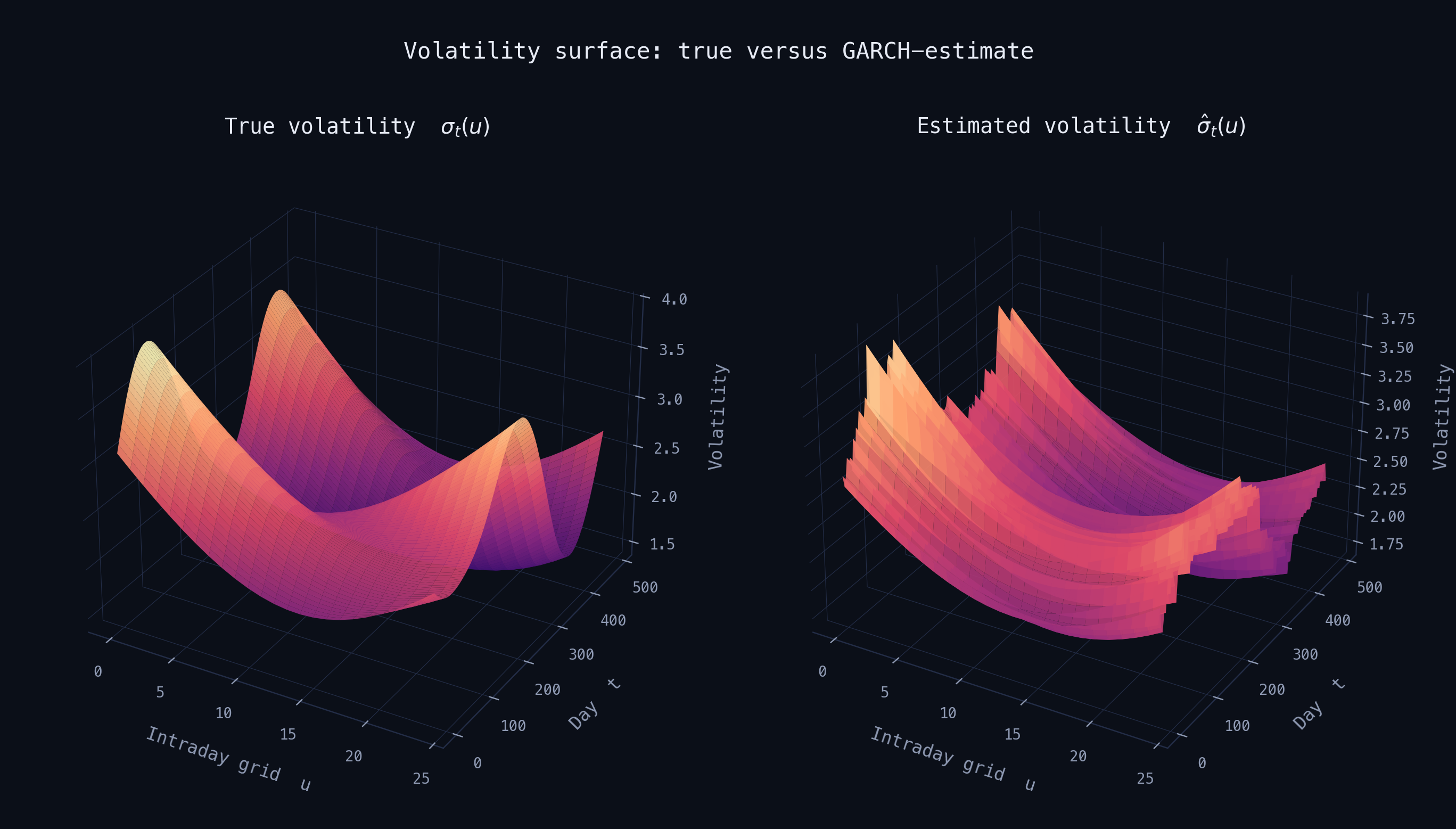
Simulated 25-point intraday grid over 500 trading days. Estimated surface via funcgarch.garch.fit + garch_filter.
It gets the main shape right. The day-to-day roughness left over comes from finite-sample noise and the limited flexibility of a basis with only three functions, not from a mistake in the estimator.
Next, the same true surface against the diagonal GAS-GARCH fit from step 3 above, using the same simulated data.
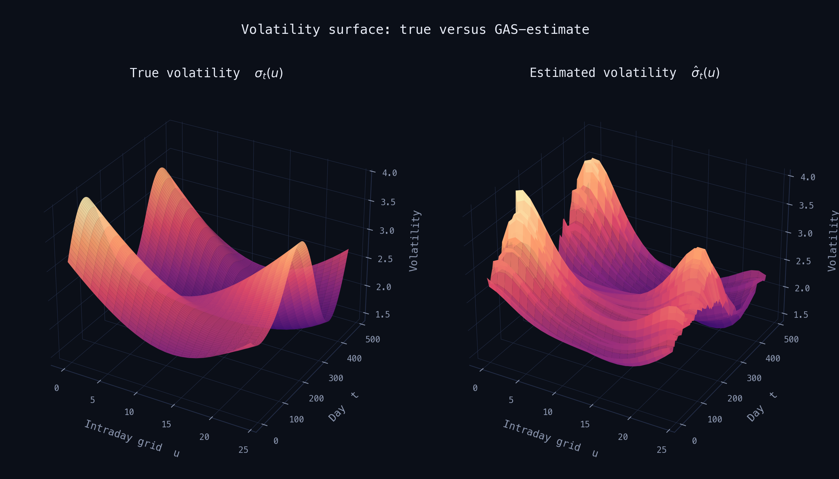
The GAS-GARCH volatility surface against the true surface, assessing recovery of the underlying dynamics.
The goodness_of_fit checks from step 4 back this up directly: the standardised residuals land
close to their theoretical Student-\(t\) moments, and the Kolmogorov–Smirnov test doesn't reject.
Because the score-driven update adapts its B-spline coefficients every day, instead of fitting one static
operator to the whole sample, this fit tracks the true surface more tightly than the plain GARCH fit above.
Finally, put the two fitted surfaces next to each other directly, instead of each against the truth separately. This makes the score-driven adaptation's smoothing effect easier to see.
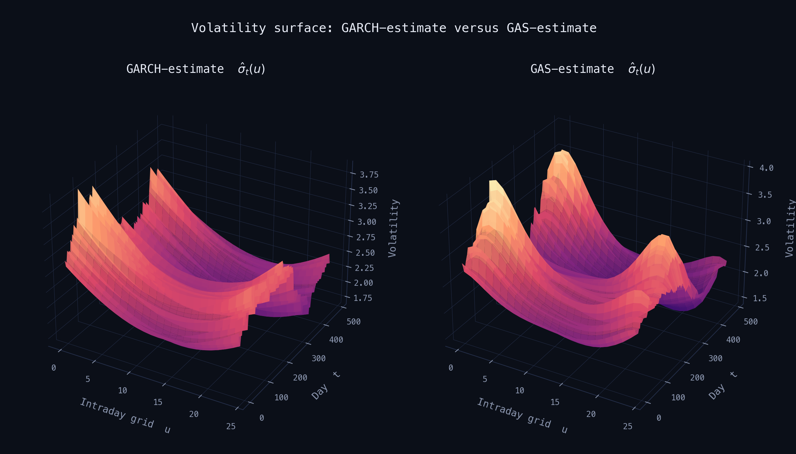
Functional GARCH versus GAS-GARCH, showing the increased flexibility of the score-driven specification.
This is exactly what the theory predicts. A static functional GARCH operator, however well fit, is a single point in operator space. It can't track a surface whose shape itself evolves. A score-driven update, by construction, adjusts its basis coefficients every day in the direction that locally improves the fit to the latest observation, and the outlier-downweighting mechanism built into the Student-\(t\) score keeps that adaptation from overreacting to any single noisy day. In Lin & Lucas's own empirical applications, intraday volatility of Pfizer stock during the COVID-19 pandemic and PM2.5 concentrations from sparse, noisy citizen-science sensors across Europe, the same robust score-driven mechanism outperforms the non-robust functional GARCH benchmark specifically during periods of market or measurement stress. That's the empirical signature of the theoretical robustness result: outlying observations get downweighted in the parameter update, rather than absorbed uncritically into the fitted surface.
Data Flow
Intraday trades are pulled from WRDS TAQ, cleaned and reshaped into the return matrix mY, and
then passed into the estimators above. The funcgarch core stays fully decoupled from this
pipeline. It never imports anything WRDS- or TAQ-specific, only ever consuming a plain numpy matrix.
wrds/*.sas                    scripts/taq_cleaner.py           funcgarch/* + scripts/gas_vol_surface.py
┌─────────────────┐           ┌────────────────────┐           ┌──────────────────────┐
│ WRDS TAQ pull   │  raw CSV  │ DataCleaner.clean()│  mY (N,T) │ fit() / garch_filter │
│ (data_fetcher,  │ ────────► │  - align to grid   │ ────────► │ fit_gas / _gas_filter│
│  taq_cleaner,   │           │  - compute returns │           │                      │
│  nbbo/dynamic_  │           │  - reshape to      │           │  -> vtheta_hat,      │
│  taq_minute,    │           │    (N, T) matrix   │           │     sigma_hat        │
│  export)        │           │                    │           │                      │
└─────────────────┘           └────────────────────┘           └──────────────────────┘
Requires Python ≥ 3.9. Pytest smoke tests cover Bernstein partition-of-unity, positive-definiteness of the OU kernel, and shape/finiteness of the GARCH filter output.