
Python · SAS · Bash
Context & Motivation
This project is the estimation and implementation side of an ongoing collaboration with André Lucas and Yicong Lin on observation-driven dynamics for functional location-scale models. The goal of the codebase is narrow. Build a fast, numerically stable estimator for a single functional GARCH(1,1) recursion, cheap enough to re-run thousands of times inside a Monte Carlo study or a rolling forecast exercise. It is the direct precursor to the Functional Volatility Surface Modelling project, which reuses the same Bernstein-basis machinery but replaces the static GARCH recursion with a score-driven update over a B-spline basis.
Computational scalability is a genuine bottleneck here, not a footnote. A functional GARCH model does not estimate a handful of scalars the way a classical GARCH(1,1) does. It estimates operators mapping curves to curves, objects that are in principle infinite-dimensional. Every evaluation of the objective function rebuilds these operators from the current parameter guess, materialises them as dense kernel matrices on the intraday grid, and runs the variance recursion through the full sample of trading days. If the grid has \(N\) intraday points, each recursion step is an \(N\times N\) matrix-vector product, and the optimizer needs thousands of function evaluations to converge, so that cost is paid thousands of times over. Keeping the per-evaluation cost small is what makes the whole approach usable, hence the JIT-compiled kernel builders, the vectorised recursion, and the separation between what can be cached across time steps and what genuinely changes every day.
Theoretical Framework
The theoretical foundation for this project is the functional GARCH quasi-maximum-likelihood framework of Cerovecki, Francq, Hörmann & Zakoïan (2018, MPRA Paper No. 83990). We work in the Hilbert space \(H = L^2([0,1])\) of square-integrable functions on the unit interval, and write \(\mathcal{K}^+(H)\) for the non-negative kernel operators on \(H\). An operator \(\alpha \in \mathcal{K}^+(H)\) acts on a curve \(x \in H\) by \(\alpha(x)(u) = \int K_{\alpha}(u,v)x(v)\,dv\) for a non-negative kernel \(K_{\alpha}\).
Write \(y_t(u)\) for the log-return at intraday time \(u \in [0,1]\) on trading day \(t\). Each day contributes a whole curve rather than a single number, which is what makes the estimation problem functional rather than scalar. A functional GARCH\((p,q)\) process is a stationary solution of \[y_t = \sigma_t \eta_t, \qquad \sigma_t^2 = \delta + \sum_{i=1}^q \alpha_i(y_{t-i}^2) + \sum_{j=1}^p \beta_j(\sigma_{t-j}^2),\] where \(\eta_t\) is an i.i.d. sequence of innovation curves, \(\delta\) is a strictly positive intercept curve, and \(\alpha_i,\beta_j \in \mathcal K^+(H)\) are non-negative kernel operators. It is the functional analogue of a classical GARCH recursion. The intercept, the ARCH and GARCH coefficients, and the conditional variance itself are now curves or operators acting on curves, not numbers.
The shape of the kernel \(K_{\alpha}\) controls how shocks propagate across intraday time. A constant kernel makes today's volatility depend on yesterday's integrated volatility only, uniformly across the day. A kernel that is peaked around the diagonal instead makes today's volatility at time \(u\) depend mainly on yesterday's volatility around the same time of day, a much more realistic intraday persistence pattern. Recovering this shape, together with the shape of \(\delta\), from data is the job of the estimation procedure below. Existence of a stationary solution is governed by a top Lyapunov exponent condition analogous to the scalar GARCH case, strictly milder than the earlier sufficient conditions of Aue, Horváth & Pellatt (2016).
The operators \(\alpha_i,\beta_j\) live in an infinite-dimensional space, so they cannot be estimated directly from a finite sample of days, and every operator must keep the variance curve positive. We solve both problems by projecting each operator onto a small set of \(M\) linearly independent, non-negative basis functions \(\varphi_1,\dots,\varphi_M \in H\), \[\delta = \sum_{k=1}^M d_k \varphi_k, \qquad \alpha_i = \sum_{k,\ell=1}^M a^{(i)}_{k,\ell}\,\varphi_k \otimes \varphi_\ell, \qquad \beta_j = \sum_{k,\ell=1}^M b^{(j)}_{k,\ell}\,\varphi_k \otimes \varphi_\ell.\] This turns an infinite-dimensional estimation problem into a finite one, over the coefficient vector \(\theta = \mathrm{vec}(d, A_1,\dots,A_q,B_1,\dots,B_p)\). The basis used throughout this codebase is the Bernstein polynomial basis, \(M\) polynomials on \([0,1]\), each non-negative everywhere on that interval. If the coefficients are all non-negative, the resulting intercept and kernel operators are automatically non-negative, so the fitted variance curve is automatically non-negative. Positivity is enforced by construction rather than by constraining the optimizer. Bernstein polynomials are a special case of B-splines, and are also the basis used in Cerovecki et al.'s own empirical study. The Functional Volatility Surface Modelling project swaps in a general B-spline basis for its score-driven extension.
Estimation & Methodology
A likelihood cannot be written down directly for a process taking values in \(H\), so the usual quasi-maximum-likelihood machinery does not carry over as is. Cerovecki et al. instead define an estimator inspired by classical GARCH QMLE. It projects the squared process onto the same basis functions used to parametrise the operators, and scores the fit with a Gaussian-QMLE-style criterion evaluated on those projections, \[\widehat\theta_n = \operatorname*{argmin}_{\theta \in \Theta} \frac1n\sum_{t=1}^n \sum_{m=1}^M \left\{ \frac{\langle y_t^2, \varphi_m\rangle}{\langle\tilde\sigma_t^2,\varphi_m\rangle} + \log\langle\tilde\sigma_t^2,\varphi_m\rangle \right\},\] where the fitted volatility curve \(\tilde\sigma_t^2\) is generated by the same recursion as the model, started from a fixed initial curve. Because the basis functions are strictly positive and the operators are non-negative, every term in the criterion is well defined, and minimising it is a well-posed finite-dimensional problem. Under standard identifiability, moment and invertibility conditions, the estimator is strongly consistent and asymptotically normal at the usual parametric rate. The same argument, as a by-product, delivers consistency and asymptotic normality for semi-strong multivariate CCC-GARCH models, since the finite-dimensional projection is exactly a multivariate CCC-GARCH representation of the functional model.
In practice the recursion is discretised on a uniform intraday grid of \(N\) points. Inner products become Riemann sums, and a kernel-operator application becomes a matrix-vector product against the \(N\times N\) matrix obtained by evaluating the kernel on the grid. Optimisation over \(\theta\) is carried out numerically with SLSQP, using simple non-negativity box constraints on the Bernstein coefficients in place of the abstract non-negativity requirement on the operators.
Code Structure & Walkthrough
The whole project lives in one file, funcgarch/garch.py: the Bernstein-basis functional
GARCH(1,1) model, its filter, and its estimator. Five pieces do the work, and they run in this order every
time you fit the model: build the basis functions, build the kernel operators from a parameter guess, run
the day loop, score each day's fit, then hand the whole thing to an optimizer. The walkthrough below follows
that order. At each step, the question is the same one: is this piece worth JIT-compiling with Numba, or is
it better left as plain NumPy calling into BLAS?
Step 1. The Bernstein basis
bernstein_basis computes \(\varphi_k^M(u) = \binom{M-1}{k-1}u^{k-1}(1-u)^{M-k}\), one Bernstein
polynomial from the theory above. It gets called \(O(M)\) times per grid point, on every single evaluation of
the objective function. That's a scalar-heavy Python loop with no matrix algebra to hand off to BLAS, exactly
the shape of code Numba is built for. It's decorated with @jit(nopython=True), Numba's
nopython mode: compile to machine code, no fallback to the slow Python interpreter if
compilation fails. This is the same as the shorthand @njit used elsewhere in the package. One
catch: Numba can't call SciPy's comb, since it only compiles a restricted subset of Python and
NumPy. So the binomial coefficient is hand-rolled from factorials instead.
@jit(nopython=True)
def bernstein_basis(u: typing.Any, n_basis: int, k: int) -> float:
    def factorial(n):
        p = 1
        for i in range(1, n + 1):
            p *= i
        return p

    def comb(n, v):
        return factorial(n) / (factorial(v) * factorial(n - v))

    degree = n_basis - 1
    v = k - 1
    return comb(n_basis - 1, k - 1) * (u ** v) * (1 - u) ** (degree - v)
delta, the level operator, uses the same basis function to build \(\delta(u) = \sum_{k=1}^M c_k
\varphi_k^M(u)\), a single sum rather than a double one. It accumulates its \(M\) terms into an
init array passed in by the caller, instead of allocating a new array itself. Numba's
nopython mode is strict about array shapes, and this trick lets the same compiled function
handle a scalar evaluation and a vectorised one over the whole intraday grid.
@njit
def delta(coefs: np.ndarray, u: float, n_basis: int, init: float = 0.0) -> float:
    """Level operator delta(u) = sum_{k=1}^M c_k * phi_k^M(u)."""
    acc = init
    for k, c in enumerate(coefs):
        acc = acc + c * bernstein_basis(u, n_basis, k + 1)
    return acc
Step 2. Building the kernel operators
kernel_operator builds the dense \(N\times N\) kernel matrix as a sum of \(M^2\) rank-one outer
products of Bernstein column vectors, the double sum behind \(\alpha_i,\beta_j\) in the theory above, now
written out on a grid. It's also JIT-compiled, for the same reason as bernstein_basis: a nested
Python loop over \(k,j \in \{1,\dots,M\}\), which Numba turns into a tight compiled loop instead of paying
interpreter overhead \(M^2\) times per call.
@jit(nopython=True)
def kernel_operator(
    u: np.ndarray,
    coefs: np.ndarray,
    n_basis: int,
    init: np.ndarray,
) -> np.ndarray:
    acc = init
    col = u.reshape((len(u), 1))
    idx = 0
    for k in range(1, n_basis + 1):
        bk = bernstein_basis(col, n_basis, k)
        for j in range(1, n_basis + 1):
            acc = acc + coefs[idx] * bk @ bernstein_basis(col, n_basis, j).T
            idx += 1
    return acc
_build_operators ties the basis functions to a specific parameter guess. It slices a flat
parameter vector into the delta, alpha and beta coefficient blocks, then calls the compiled basis functions
exactly once to build delta_hat, alpha_hat and beta_hat as plain
grid-space arrays. This is the boundary between the JIT-compiled code above and the plain NumPy day loop
below. Every day in that loop reuses these same three arrays instead of touching the basis functions again.
Rebuilding an \(N\times N\) kernel matrix costs \(O(N^2 M^2)\). Paying that cost once per optimizer step,
instead of once per day, over hundreds of trading days, is the single biggest win in the whole pipeline.
def _build_operators(
    params: np.ndarray,
    n_basis: int,
    n_grid: int,
    delta_fn: typing.Callable,
    kernel_fn: typing.Callable,
) -> tuple[np.ndarray, np.ndarray, np.ndarray, np.ndarray]:
    grid = np.linspace(1 / n_grid, 1 - 1 / n_grid, n_grid)
    delta_coefs = params[:n_basis]
    alpha_coefs = params[n_basis: n_basis + n_basis ** 2]
    beta_coefs  = params[n_basis + n_basis ** 2:]
    delta_hat = delta_fn(delta_coefs, grid, n_basis=n_basis, init=np.zeros(n_grid))
    alpha_hat = kernel_fn(grid, alpha_coefs, n_basis=n_basis, init=np.zeros((n_grid, n_grid))).T
    beta_hat  = kernel_fn(grid, beta_coefs,  n_basis=n_basis, init=np.zeros((n_grid, n_grid))).T
    return grid, delta_hat, alpha_hat, beta_hat
Step 3. Running the day loop
With delta_hat, alpha_hat and beta_hat fixed, the recursion
\(\sigma_t^2 = \delta + \alpha(y_{t-1}^2) + \beta(\sigma_{t-1}^2)\) becomes a simple loop over trading days.
Each integral turns into an elementwise-weighted matrix-vector product, divided by the grid size. This loop
is, on purpose, not JIT-compiled. Its cost per iteration is dominated by \(N\times N\)
matrix-vector products, and NumPy already sends that work to BLAS, a hand-tuned, multi-threaded
linear-algebra library that Numba's own compiled code can't beat. Compiling a loop whose real cost sits
inside a BLAS call would add compile time for no speed gain. It would also stop the loop from calling
loss_fn as an ordinary Python function, and garch_estimator needs that flexibility,
since delta_fn, kernel_fn and loss_fn can all be swapped for a
different basis.
for t in range(1, n_days):
    variance = (
        delta_hat
        + ((alpha_hat * returns[:, t - 1] ** 2) @ np.ones(n_grid_obs)
        +  (beta_hat  * variance)               @ np.ones(n_grid_obs)) / n_grid_obs
    )
    total_loss += loss_fn(returns[:, t], variance, n_basis, grid)
Step 4. Scoring each day's fit
loss_func computes a Bernstein-projected mean squared error between the squared returns and the
fitted variance, summed across the \(M\) basis functions,
\(L_t = \sum_{k=1}^M \frac1N\sum_i \bigl[(y_t^2(u_i)-\sigma_t^2(u_i))\varphi_k^M(u_i)\bigr]^2\). It's a
cheaper stand-in for the formal QMLE criterion from the theory section, trading some statistical efficiency
for something fast to evaluate and easy to differentiate numerically. This one is JIT-compiled too. It loops
over the \(M\) basis functions on every single day, so it runs \(M\) times a day, times hundreds of days,
times thousands of optimizer evaluations. That's where the interpreter overhead would add up fastest if left
uncompiled.
@jit(nopython=True)
def loss_func(
    returns: np.ndarray,
    variance: np.ndarray,
    n_basis: int,
    grid: np.ndarray,
) -> float:
    total = 0.0
    for k in range(1, n_basis + 1):
        w = bernstein_basis(grid, n_basis, k)
        total += np.mean(((returns ** 2 - variance) * w) ** 2)
    return total
Step 5. Fitting the model
garch_estimator wraps the day loop above and returns a single scalar loss, the thing
scipy.optimize.minimize actually needs. garch_filter runs the identical recursion
but returns the full (n_grid, n_days) variance surface instead, and is used once fitting is
done, to recover the fitted volatility surface for the whole sample. fit sits on top of both: a
thin wrapper around scipy.optimize.minimize that closes over the data and hyperparameters, so
the optimizer only ever sees a function of the parameter vector.
def fit(
    returns: np.ndarray,
    initial_variance: np.ndarray,
    n_grid: int,
    n_basis: int = 1,
    estimator_fn: typing.Callable = garch_estimator,
    delta_fn: typing.Callable = delta,
    kernel_fn: typing.Callable = kernel_operator,
    loss_fn: typing.Callable = loss_func,
    print_convergence: bool = False,
    options: dict | None = None,
    **kwargs,
) -> ResultContainer:
    def _objective(params: np.ndarray) -> float:
        return estimator_fn(
            returns, n_grid, params,
            n_basis=n_basis, initial_variance=initial_variance,
            delta_fn=delta_fn, kernel_fn=kernel_fn, loss_fn=loss_fn,
            print_convergence=print_convergence,
        )

    opt = minimize(_objective, options={'disp': True, **(options or {})}, **kwargs)
    return ResultContainer(**{k: opt[k] for k in opt.__dir__()})
Non-negative Bernstein coefficients guarantee a positive volatility surface directly, without constrained optimization over the full operator. ResultContainer is a small key-value wrapper that exposes every field of the underlying scipy.optimize.OptimizeResult as an attribute, so result.x, result.fun and result.success all work as expected.
Putting it together, fitting the model and recovering the surface takes two calls. x0 and
bounds are laid out as
[delta_coefs (n_basis) | alpha_coefs (n_basis²) | beta_coefs (n_basis²)], matching the
slicing inside _build_operators above.
n_basis = 4
n_params = n_basis + 2 * n_basis ** 2

result = fit(
    returns, initial_variance=np.ones(n_grid), n_grid=n_grid, n_basis=n_basis,
    x0=np.zeros(n_params),
    bounds=[(-0.99, 0.99)] * n_params,
    method='SLSQP',
)
sigma2_hat = garch_filter(
    returns, n_grid=n_grid, params=result.x, n_basis=n_basis,
    initial_variance=np.ones(n_grid),
)
Results & Empirical Discussion
Running steps 1 to 5 on simulated intraday data, generated from a known functional GARCH(1,1) recursion via
funcgarch.simulate.simulate (which reuses the same Bernstein operator builders as the estimator
itself), gives the fitted volatility surface below, using M = 3 basis functions.
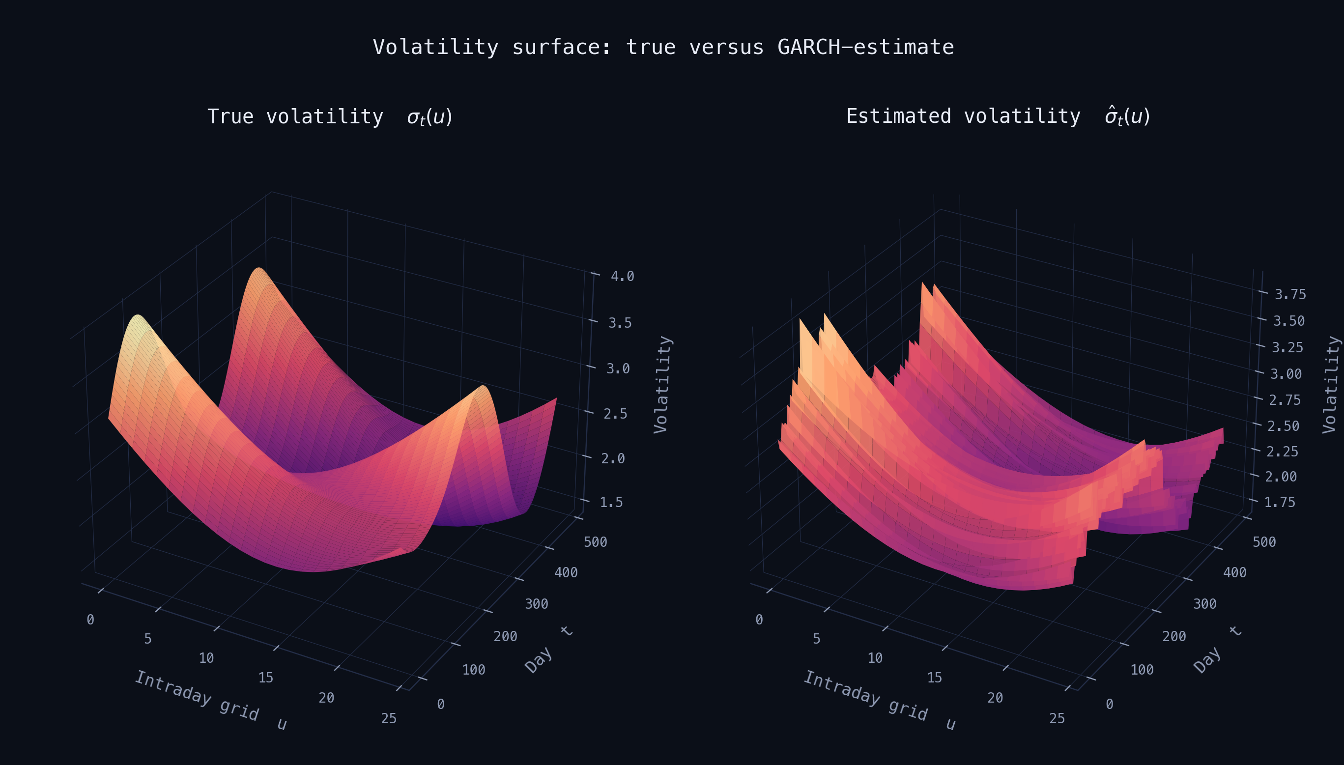
Simulated 25-point intraday grid over 500 trading days. Estimated surface via funcgarch.garch.fit + garch_filter.
The estimation recovers the main structure of the true process. The remaining day-to-day roughness comes from finite-sample effects and the limited flexibility of a basis with only three functions, not from a flaw in the estimator.
This mirrors the theoretical picture from the underlying paper's own simulation study. On a functional GARCH(1,1) with a low-dimensional true kernel spanned by the fitting basis, the QMLE cuts both standard deviation and bias by roughly a factor of 2–3, relative to the least-squares estimator of Aue, Horváth & Pellatt (2016). It stays close to its target even when the instrumental functions are chosen by a data-driven functional-PCA-style routine, rather than fixed in advance. That's empirical confirmation that the consistency and asymptotic normality guarantees above hold at realistic sample sizes, not just asymptotically.
In the real-data application to the S&P100 index, the fitted volatility curves track both the sensitivity of volatility to shocks at the intraday scale and its day-to-day persistence. The corresponding one-day-ahead realised-volatility forecasts, obtained by summing the predicted variance curve over the intraday grid, track the true realised volatility closely across sample periods of varying turbulence. That is the practical payoff of having an estimator fast enough to actually run this recursion on ten years of minutely data.