Functional Volatility · Market Microstructure · Dynamic Modelling

Experience & Projects_

Roles and side projects at the intersection of statistics, execution, and market-making.

The complete resume, plus the projects behind it. Expand any project for an overview and a code sketch.

Work Experience

QuantFi · Quantitative Developer

Schiphol-Rijk, Netherlands

Built and deployed algorithmic market-making strategies: volatility/skew estimation, order-flow modelling, queue-aware execution, and reference-price dynamics. Alongside quoting, I built a dynamic liquidity allocation model for smart order routing across fragmented order books, cutting slippage and transaction costs by an average of 5.8%, and cross-exchange rebalancing methods that time inventory transfers under latency, funding-rate, and liquidity constraints.

Python · asyncio · numba · ccxt

Overview

Market making can be formulated as a stochastic optimal-control problem: choose bid and ask quotes around a reference price to maximize expected spread capture while controlling inventory risk. In the Guéant–Lehalle–Fernandez-Tapia framework, the reference price follows a diffusion \[dS_t = \sigma dW_t,\] while order arrivals depend on quote distance through \[\lambda(\delta) = Ae^{-k\delta}.\] Solving the control problem gives the theoretical optimal quotes. In the finite-horizon Avellaneda–Stoikov model, \[\delta_t^{b*} = \frac{1}{\gamma}\log(1+\gamma/k) + \frac{1+2q_t}{2}\gamma\sigma(T-t),\] and \[\delta_t^{a*} = \frac{1}{\gamma}\log(1+\gamma/k) + \frac{1-2q_t}{2}\gamma\sigma(T-t),\] where the first term represents the baseline spread and the second term skews quotes according to inventory. For continuous markets such as crypto, the infinite-horizon Guéant formulation removes the terminal-time dependence and yields stationary quotes determined by inventory, volatility, liquidity, and risk aversion. In practice, these models are extended with dynamic volatility estimates, order-flow signals, queue-position models, latency-aware execution, and exchange-specific risk controls.

Python code: async quote-management loop illustrating live deployment:

async def market_maker(feed, exchange, model):
    while True:
        market = await feed.next_update()

        state = {
            "mid": market.mid,
            "inventory": await exchange.inventory(),
            "volatility": market.volatility,
        }

        quotes = model.compute_quotes(state)

        await exchange.cancel_stale_orders()
        await exchange.place_quotes(quotes)

        await asyncio.sleep(0.01)

Illustrative formulation of the class of technique; production market-making systems typically use proprietary calibration, execution models, risk controls, and infrastructure.

VU Econometrics and Data Science · Research Assistant

Amsterdam, Netherlands

Collaborated with Yicong Lin and Andre Lucas on robust observation-driven dynamics for functional location-scale models (see Publications). My contribution focused on the estimation and implementation of the functional volatility component: by projecting infinite-dimensional conditional-variance operators onto a finite Bernstein-polynomial basis, the positivity-constrained QMLE problem is reduced to a bounded, finite-dimensional optimization. The implementation constructs the functional operators, performs the volatility recursion, and estimates the model parameters through constrained likelihood optimization:

def bernstein_basis(u, M, k):
    return comb(M - 1, k - 1) * u ** (k - 1) * (1 - u) ** (M - k)

def functional_operator(grid, coefs, M):
    phi = np.stack([bernstein_basis(grid, M, k) for k in range(1, M + 1)])
    return sum(c * np.outer(phi[i], phi[j]) for c, (i, j) in zip(coefs, product(range(M), repeat=2)))

def qmle_filter(returns, theta, M):
    delta, alpha, beta = theta[:M], theta[M:M + M**2], theta[M + M**2:]
    grid = np.linspace(0, 1, returns.shape[0])
    A, B = functional_operator(grid, alpha, M), functional_operator(grid, beta, M)
    d = sum(c * bernstein_basis(grid, M, k) for k, c in enumerate(delta, 1))

    sigma2 = np.ones(returns.shape[0])
    surface = np.zeros_like(returns)
    for t in range(1, returns.shape[1]):
        sigma2 = d + (A @ returns[:, t - 1] ** 2 + B @ sigma2) / returns.shape[0]
        surface[:, t] = sigma2
    return surface

theta_hat = minimize(lambda theta: qmle_loss(returns, theta, M), theta0, method='SLSQP').x

Non-negative Bernstein coefficients guarantee a positive volatility surface directly, without constrained optimization over the full operator.

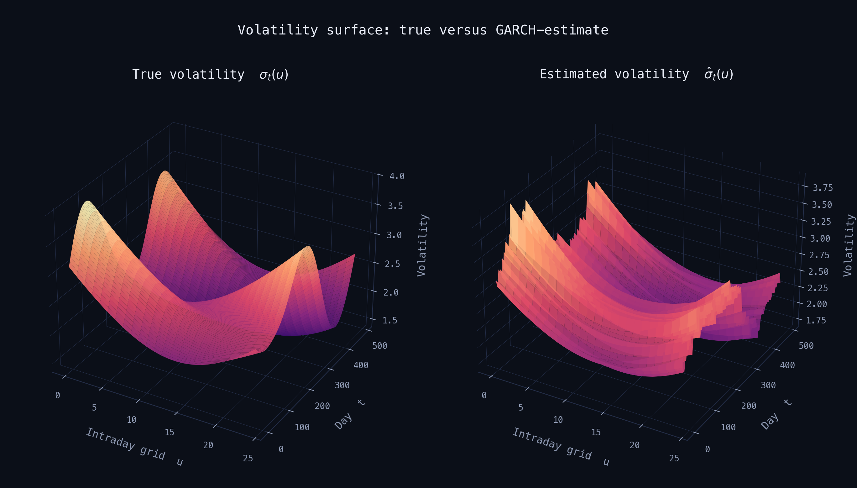
Applying this framework to simulated intraday data with a functional GARCH(1,1) recursion and Bernstein-basis QMLE with M = 3 basis functions gives the fitted volatility surface shown below. The estimation recovers the main structure of the true process, while the remaining day-to-day roughness reflects finite-sample effects and the limited flexibility of the chosen basis:

True versus functional GARCH-estimated volatility surface, side by side

Simulated 25-point intraday grid over 500 trading days; estimated surface via funcgarch.garch.fit + garch_filter.

QuantFi · Operational Trader

Schiphol-Rijk, Netherlands

Monitored production market-making algorithms, managing real-time risk parameters and system health to limit inventory exposure through high-volatility periods. Designed and deployed a live trading terminal on ccxt and native exchange APIs for real-time position and order tracking, integrating Tardis.dev to reconstruct historical positions from raw fills when a session needed to be audited after the fact.

Python · ccxt · Tardis.dev

Projects

Functional Volatility Surface Modelling

  • Extending the functional GARCH framework to a generalized autoregressive score (GAS) model to estimate and capture time-varying intraday volatility surfaces.
  • Designed efficient estimation procedures using B-splines, applying numba JIT compilation to enable scalable modelling of volatility surfaces from granular intraday return data.
Python · SAS · FunctionalScale on GitHub

Overview

Treats continuous intraday log-return paths as functional data objects \(y_t(u)\) over the trading day \(u \in [0,1]\). The Functional GARCH(p,q) model generalizes classical volatility dynamics to an infinite-dimensional Hilbert space, capturing how shocks at any point of the day impact the entire upcoming volatility surface.

Model Definition

The functional scale model decomposes returns using a time-varying conditional variance curve \(\sigma_t^2(u)\), so we look at \[y_t(u) = \sigma_t(u)\eta_t(u)\] driven by the recursion \[\sigma_t^2 = \delta + \sum_{i=1}^{q}\alpha_i\left(y_{t-i}^2\right) + \sum_{j=1}^{p}\beta_j\left(\sigma_{t-j}^2\right)\]

where \(\delta\) is a strictly positive baseline intercept curve, and \(\alpha_i, \beta_j\) are non-negative integral kernel operators mapping past squared return curves and past volatility curves into today's volatility surface.

Functional GAS Extension

The functional scale model can be extended to a functional Generalized Autoregressive Score (GAS) model by replacing the autoregressive dependence on past squared return curves with a score-driven update. The returns are defined as \[y_t(u) = \sigma_t(u)\eta_t(u),\] where \(\sigma_t^2(u)\) denotes the time-varying conditional variance curve. The functional GAS dynamics are specified as \[\sigma_{t+1}^2 = \delta + B\sigma_t^2 + A\int \phi_K(s)y_t^2(s)\,ds,\] where \(\delta\) is a strictly positive baseline intercept curve, \(B\) is a linear persistence operator acting on the previous volatility curve, and \(A\) maps the observed squared return curve into the updated volatility curve. The basis projection term \[\int \phi_K(s)y_t^2(s)\,ds\] represents the score-driven innovation component obtained from the functional representation of the return process.

Equivalently, the recursion can be expressed using integral kernel operators as \[\sigma_{t+1}^2(u) = \delta(u) + \int B(u,v)\sigma_t^2(v)\,dv + \int A(u,s)\phi_K(s)y_t^2(s)\,ds.\] The functional GAS model therefore updates the conditional variance curve using information contained in the most recent squared return curve, while the operator \(B\) captures the persistence of past volatility curves. Compared with the functional scale model, \[\sigma_t^2 = \delta + \sum_{i=1}^{q}\alpha_i(y_{t-i}^{2}) + \sum_{j=1}^{p}\beta_j(\sigma_{t-j}^{2}),\] the GAS formulation replaces the ARCH-type feedback operators \(\alpha_i(y_{t-i}^{2})\) with a score-driven update based on the functional projection of the return innovations.

Estimation

Because standard likelihood functions cannot be directly evaluated for continuous curves, the model is estimated using Functional Quasi-Maximum Likelihood Estimation (QMLE).

Setup

git clone https://github.com/DaanZunnenberg/FunctionalScale.git
cd FunctionalScale
pip install -e .            # editable install, pulls in numpy/scipy/numba/pandas/matplotlib/tqdm
pip install -e ".[dev]"      # + pytest, jupyter (optional, for tests/notebooks)

Usage: functional GARCH

import numpy as np
from funcgarch import fit, garch_filter

# mY: (N, T) matrix of intraday return curves, N grid points per day, T days
mY = np.load("returns.npy")
N, T = mY.shape
M = 4  # number of Bernstein basis functions

result = fit(mY, n_grid=N, M=M)          # QMLE-style estimation (scipy.optimize)
vtheta_hat = result.x

sigma2 = garch_filter(mY, n_grid=N, vtheta=vtheta_hat, M=M)  # (N, T) fitted variance surface

Usage: functional GAS-GARCH

from scipy.optimize import minimize
from funcgarch import gas_garch_estimator

# vtheta = [nu, ou_scale, omega (M,), vec(B) (M*M,), vec(A) (M*M,)]
result = minimize(
    gas_garch_estimator, x0=vtheta_init, args=(mY, N, M),
    method="SLSQP",
)

Because the score-driven update adapts its B-spline coefficients every day rather than fitting one static operator to the whole sample, the GAS-GARCH fit tracks the true surface considerably more tightly than the plain functional GARCH fit above:
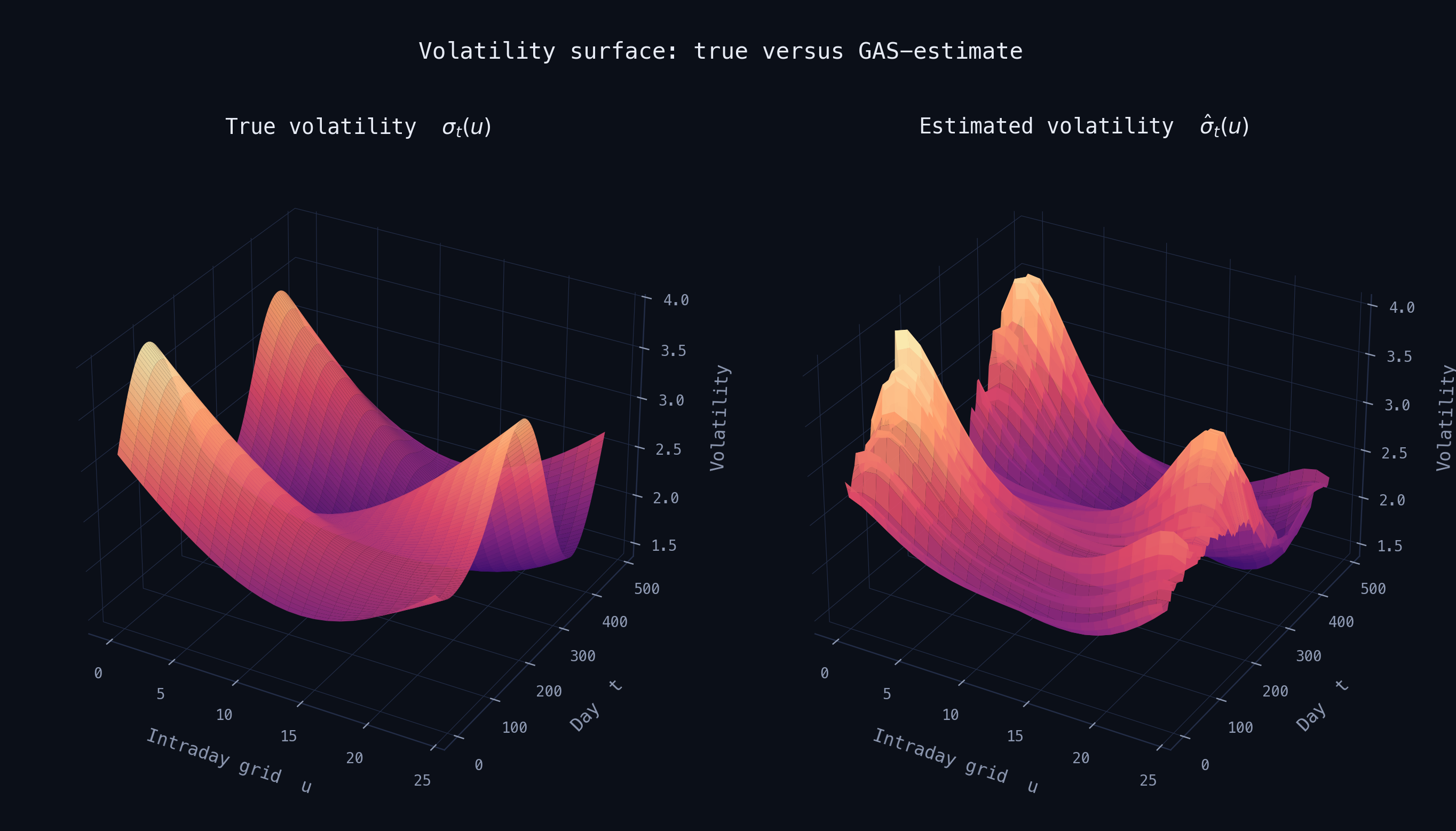
True versus GAS-GARCH-estimated volatility surface, side by side

The first comparison figure shows the estimated GAS-GARCH volatility surface against the true volatility surface to assess the model’s ability to recover the underlying dynamics.

Placing the two estimators' fitted surfaces directly next to each other, rather than each against the true surface separately, makes the score-driven adaptation's smoothing effect easier to see:
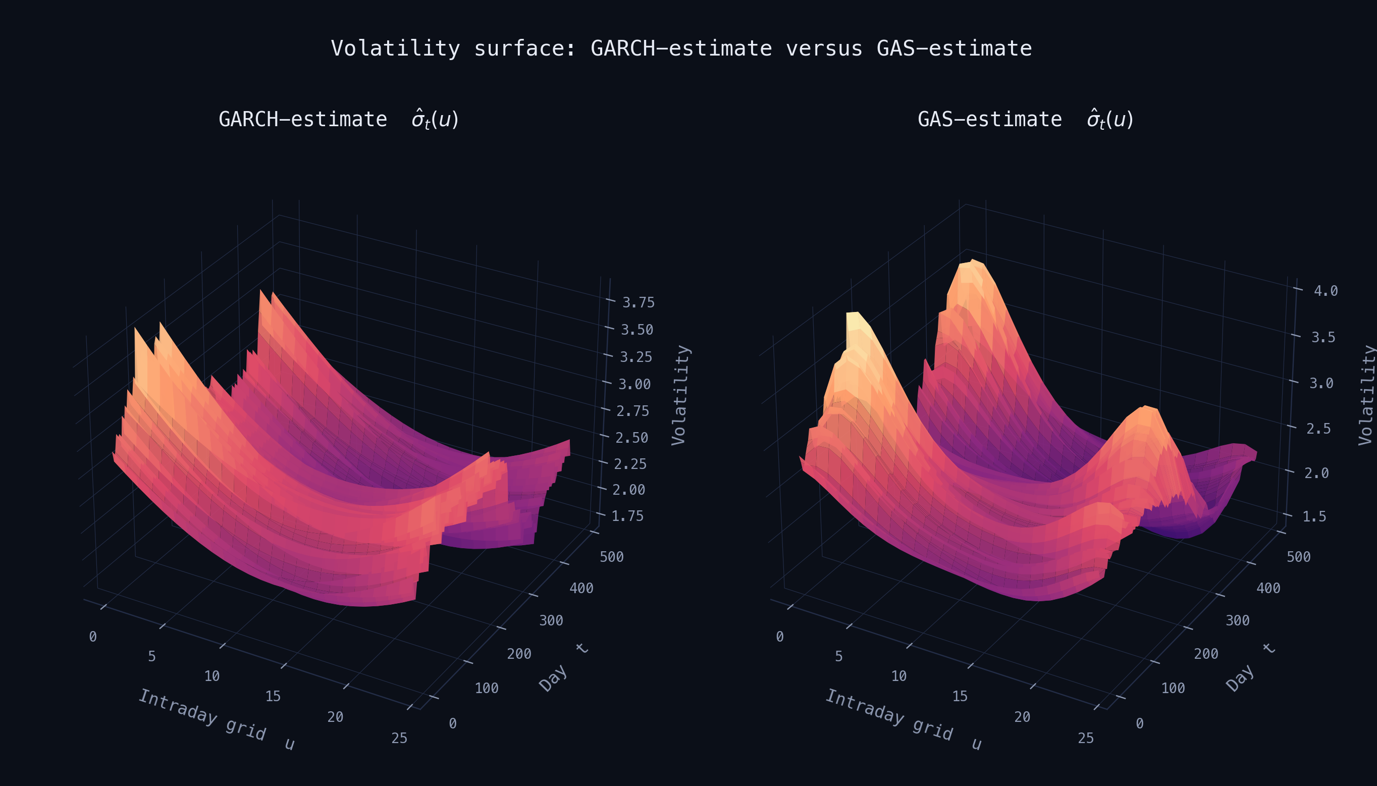
Functional GARCH-estimated versus GAS-GARCH-estimated volatility surface, side by side

The second comparison figure compares the functional GARCH and GAS-GARCH volatility surfaces, demonstrating the increased flexibility of the GAS-GARCH specification relative to the traditional functional GARCH model.

Data Flow

wrds/*.sas                    scripts/taq_cleaner.py           funcgarch/*.py
┌─────────────────┐           ┌────────────────────┐           ┌──────────────────────┐
│ WRDS TAQ pull   │  raw CSV  │ DataCleaner.clean()│  mY (N,T) │ fit() / garch_filter │
│ (data_fetcher,  │ ────────► │  - align to grid   │ ────────► │ gas_garch_estimator  │
│  taq_cleaner,   │           │  - compute returns │           │ func_garch_estimator │
│  nbbo/dynamic_  │           │  - reshape to      │           │                      │
│  taq_minute,    │           │    (N, T) matrix   │           │  -> vtheta_hat,      │
│  export)        │           │                    │           │     sigma2 surface   │
└─────────────────┘           └────────────────────┘           └──────────────────────┘

Requires Python ≥ 3.9. Full theory, references, and repository layout in the README.
Functional Stationarity Test

A functional stationarity test for multidimensional diffusion processes, developed for my MSc thesis and released as an open-source library.

Overview

We consider a d-dimensional Itô diffusion process \((X_t)_{t \ge 0}\) defined by \[dX_t = b(X_t)\,dt + \sigma(X_t)\,dW_t,\] where \(X_t \in \mathbb{R}^d\), \(b: \mathbb{R}^d \to \mathbb{R}^d\) is the drift function, \(\sigma: \mathbb{R}^d \to \mathbb{R}^{d \times m}\) is the diffusion coefficient, and \(W_t\) is an \(m\)-dimensional Brownian motion. The instantaneous covariance matrix is given by \[a(x) = \sigma(x)\sigma(x)^\top.\]

Throughout, we assume that the diffusion satisfies the uniform ellipticity condition, meaning that there exists a constant \(\lambda > 0\) such that \[\xi^\top a(x) \xi \ge \lambda \|\xi\|^2, \qquad \forall x \in \mathbb{R}^d,\ \xi \in \mathbb{R}^d.\] This assumption ensures that the diffusion is non-degenerate in every direction. As a consequence, the transition probabilities of the process assign positive probability to every non-empty open subset of the state space. Hence, the process is open-set irreducible. Moreover, under standard regularity conditions, the diffusion is aperiodic.

If the process is additionally positive Harris recurrent, then it admits a unique invariant probability distribution and satisfies the usual ergodic properties of Markov processes. In particular, long-run averages of functions of the process converge to their corresponding expectations under the invariant distribution, ensuring stable long-run behaviour.

The proposed stationarity test is based on the relationship between stationarity and the growth behaviour of the occupation measure, \[\mu_t(A) = \int_0^t \mathbf{1}_A(X_s)\,ds,\] which measures the amount of time the diffusion spends in a measurable set \(A\). For a stationary and ergodic diffusion, the occupation measure grows linearly with time, with the growth rate determined by the invariant distribution. Therefore, under the diffusion assumptions above, stationarity is equivalent to linear divergence of the occupation measure.

The test exploits this equivalence by comparing two consistent estimators of the diffusion matrix. The first estimator is constructed in the time domain, while the second estimator is constructed in the state domain using the occupation measure. Under stationarity, the linear growth of the occupation measure guarantees compatible asymptotic behaviour of both estimators. Under nonstationarity, this linear divergence property fails, leading to a divergence between the two estimators.

The limiting distribution used for the test statistic is obtained from the extreme value theory of Pickands and Berman for running maxima of stationary Gaussian sequences. Under the stationary regime, the standardized difference between the estimators admits a Gaussian approximation, and the corresponding running maximum converges to a Gumbel-type limit distribution. The critical values for the test are therefore obtained from this Pickands–Berman extreme value distribution.

Setup

pip install -e .

Or install dependencies only:

pip install -r requirements.txt

Quick Start

import numpy as np
from mht.models.processes import BivariateOUProcess
from mht.testing.kernel_test import KernelTest, Kernel, TestPlotter

# Simulate a bivariate OU process
ou_config = {
    'T': 365, 'dt': 1/20,
    'sigma1': np.sqrt(2), 'sigma2': np.sqrt(2),
    'theta1': 0.2, 'theta2': 0.2,
    'rho': 0.75,
}
process = BivariateOUProcess(**ou_config)
process.simulate(seed=1)
X, T, n = process.config()

# Set up the test configuration
config = {
    'data': X,
    'kernel_params': {
        'bandwidth': np.sqrt(3) * 9 / ((n ** (1/6)) * np.log(n)),
        'n': n, 'T': T,
        'kernel': Kernel.BaseKernel,
    },
    'time_params': {'bandwidth': 200 * T / n, 'n': n, 'T': T},
}

# Estimate and test
test = KernelTest(**config)
test.time_domain_smoother(lamb=0.99)
test.state_domain_smoother(dist=True)   # True = use KDE for joint density
test.gauss()

bound, scalar_gauss = test.transform_1D_gauss()

# Plot
plotter = TestPlotter(test)
plotter.plot_running_maximum()

Repository Structure

src/mht/
    testing/
        kernel_test.py        # KernelTest, Simulator, TestPlotter
        hypothesis.py         # MultipleHypTest, UnitRootTest, LaTeXTable
        leybourne_mccabe.py   # Leybourne-McCabe test (single canonical copy)
    models/
        processes.py          # BivariateOUProcess, BivariateCorrelatedBM, ...
    io/
        reader.py             # Reader class for simulation CSV files
    viz/                      # TestPlotter re-exported here
    utils/
        decorators.py
simulations/                  # Pre-computed CSV simulation results
notebooks/
    example.ipynb
tests/
    test_processes.py
    test_kernel_test.py

Requires Python ≥ 3.10. Also includes batch KPSS and Leybourne–McCabe tests for comparison, and BH/BY FDR procedures for simulation studies.

HRP Portfolio Allocation

  • Implemented Hierarchical Risk Parity via tree clustering using scipy.cluster to stabilize high-dimensional asset allocation, bypassing classical covariance inversion to eliminate noise sensitivity.
  • Generated a mean alpha premium of 3.9% above the benchmark across diverse simulated horizons, in a look-ahead-free method that outperformed actively rebalanced benchmark portfolios.

Overview

Mean-variance allocation is fragile in high dimensions because it inverts a noisy covariance matrix. Hierarchical Risk Parity (HRP) sidesteps the inversion entirely: assets are clustered by correlation distance, then risk is allocated recursively down the resulting tree.

Approach

Clustering uses scipy.cluster.hierarchy on a correlation-distance matrix; weights are then derived by recursive bisection down the dendrogram, splitting inverse-variance weight between each pair of sub-clusters. All backtests are look-ahead-free, re-clustering only on data available at each date.

from scipy.cluster.hierarchy import linkage, dendrogram
from hrp import correlation_distance, recursive_bisection

dist = correlation_distance(returns)
tree = linkage(dist, method="single")
order = dendrogram(tree, no_plot=True)["leaves"]

weights = recursive_bisection(returns.cov(), order)

Illustrative interface. The production version adds transaction-cost-aware rebalancing.

Dynamic Clustering with a Score-Driven HMM

Dynamic clustering of multivariate panel data: a GAS filter drives the time-varying means of an HMM-style mixture model, so cluster membership evolves rather than staying fixed.

Overview

Each unit \(i\) belongs to a latent cluster \(s_{i,t} \in \{1,\dots,K\}\), with observations \(y_{i,t} \mid s_{i,t}=k \sim \mathcal{N}(\mu_{k,t}, \Sigma_{k,t})\). The transition probabilities are shared across units and depend on the distance between cluster-specific location parameters, scaled by a sensitivity parameter \(\gamma\):

\[ \pi_t^{(j \to k)} = \frac{\exp(-\gamma\, d(\mu_{j,t-1}, \mu_{k,t-1}))}{\sum_{m=1}^K \exp(-\gamma\, d(\mu_{j,t-1}, \mu_{m,t-1}))} \]

where \(d(\cdot,\cdot)\) denotes the Mahalanobis distance.

The cluster parameters are allowed to evolve dynamically through a Generalized Autoregressive Score (GAS) recursion rather than being fixed over time. Let \(f_{k,t}\) denote the time-varying state associated with cluster \(k\). The update is given by

\[ f_{k,t+1} = \omega_k + A_k s_{k,t} + B_k f_{k,t}, \]

where the scaled score is

\[ s_{k,t} = S_{k,t}\, \frac{\partial \log p(y_t \mid f_{k,t})}{\partial f_{k,t}}. \]

This score-driven specification allows the cluster characteristics to adapt to new observations while preserving the dynamic structure of the mixture model.

Setup

git clone https://github.com/DaanZunnenberg/DynamicCluster.git
cd DynamicCluster
pip install -e .

Usage

python scripts/run_simulation.py

Simulates panel data under a known dynamic-clustering process, estimates parameters by maximum likelihood, and writes recovered vs. true cluster structure to a .csv.

Tukey Depth Under Mixing

Research code for studying Tukey depth under dependence: how depth-based statistical methods behave when observations come from dependent, mixing time series rather than independent samples.

Overview

This repository contains research code for studying Tukey depth under dependence. The objective is to investigate how depth-based statistical methods behave when observations are generated from dependent time series rather than independent samples. The code provides tools for simulating dependent, mixing time series processes and estimating Tukey's halfspace depth together with the corresponding minimal direction.

The package includes simulation routines for generating synthetic bivariate time series with different dependence structures and controllable mixing behaviour. It also provides implementations for estimating Tukey depth and the direction that determines the limiting halfspace empirically from simulated samples. In addition, the code includes closed-form benchmark cases for Gaussian models and stationary vector autoregressive processes, allowing the empirical estimates to be compared against theoretical values.

The main application is to study the convergence behaviour of depth estimates as the sample size increases under different dependence regimes.

Usage

from Core.MixingModels import MixingLinearModel
from Core.Depth import Estimator, GaussianDepth

process = MixingLinearModel(mixing_rate=1.5)
X = process.simulate(n=500)

result = Estimator(X, X0, method="deg")   # or "point_wise"
depth, direction = result.depth, result.direction

Illustrative interface. See the notebooks in Core/ for the full VAR(1) and mixing-process walkthroughs.

EUR/USD 2-Minute Bar Dataset

Free EUR/USD OHLCV data at 2-minute bars for 2025, released as a sandbox for backtests, strategy prototyping, and analysis.

Overview

One CSV per month of 2-minute EUR/USD bars (open, high, low, close, volume, trade count), covering all of 2025. Provided as-is, no rights reserved, for anyone who wants sample FX data to experiment with.

Data tools

from scripts.data_tools import load_months, load_all, resample

df = load_months(["2025-01", "2025-02"])  # combine specific months
df = load_all()                           # combine all available months
hourly = resample(df, "1h")               # resample to any pandas offset alias

Visualization

pip install -r requirements.txt
python scripts/visualize.py --all
python scripts/visualize.py --all --resample 1h

Tardis.dev Data Fetcher

A focused client for downloading historical cryptocurrency market data from Tardis.dev: authentication, layered configuration, retries, and resumable downloads.

Overview

Scoped to fetching only. FetchOptions merges CLI flags, a config file, and the TARDIS_API_KEY environment variable in that priority order; TardisClient builds Datasets API requests, authenticates, retries transient failures with backoff, and skips files that already exist unless overwriting is requested.

Setup

python3 -m venv .venv && source .venv/bin/activate
pip install -e ".[dev]"
cp .env.example .env   # then edit .env with your real key

Usage

tardis-inspect check-key
tardis-inspect exchanges
tardis-fetch --config config/example.yaml

RiskFunctions

A library of risk models organized by family: variance-covariance and historic-simulation VaR/ES, CCC-GARCH, EWMA-FHS, copulas, and factor analysis, packaged as an installable library.

Overview

Each model family under src/riskfunctions/models/ holds pure estimator/analysis functions operating on DataFrames and arrays, with no I/O or plotting baked in; anything that loads data, wires a model together, or produces output lives in examples/ instead.

Installation

python -m venv .venv
source .venv/bin/activate
pip install -e ".[dev]"          # core + test dependencies
pip install -e ".[multivariate]" # needed only for copulas / factor analysis

Usage

python examples/var_covariance_example.py
python examples/ccc_garch_example.py
python examples/ewma_fhs_example.py

Subspace-Based Time-Delay Estimation for WiFi

Subspace-based (MUSIC, ESPRIT, matrix pencil) time-delay estimation for IEEE 802.11n WiFi L-LTF signals. Research paper to be published.

Overview

The L-LTF preamble of a WiFi packet is a known training sequence, so a receiver's channel estimate is a sum of delayed, attenuated copies of it, one per multipath tap. Time-delay estimation recovers those delays directly from the channel/frequency response rather than from cross-correlation alone. MUSIC gets there by eigendecomposing the array/frequency covariance matrix into a signal subspace and a noise subspace, then scanning candidate delays for the ones whose steering vector is (almost) orthogonal to the noise subspace, using the pseudo-spectrum

\[ P(\tau) = \frac{1}{a(\tau)^{H} \, E_n E_n^{H} \, a(\tau)} \]

where \(a(\tau)\) is the steering vector for delay \(\tau\) and \(E_n\) collects the noise-subspace eigenvectors, so \(P(\tau)\) peaks sharply at the true delays. ESPRIT and matrix pencil solve the same subspace-separation problem without an explicit search, by exploiting a shift-invariance structure in the signal subspace instead.

Install

pip install -e .

Run

python examples/basic_usage.py
python scripts/run_tde.py

src/musicssvd/ separates signal generation (DataGenerator), TDE algorithms (DataProcessor), accuracy metrics (Evaluator), and plotting (Plotter), wired together by the MUSICTDE facade.

More on GitHub.

Education

Leiden University

Doctor of Philosophy (PhD), Mathematics · Leiden, Netherlands

Researching decomposition theorems, generic chaining, and majorizing measures for controlling suprema of stochastic processes, applied to weak convergence and Donsker–Skorokhod-type results under absolute regularity. I also organize and lead a weekly graduate seminar on weak convergence and empirical process theory. The full technical writeup, including a walkthrough of the \(\gamma_2\) functional and the majorizing measure theorem, is on the Research page.

Vrije Universiteit Amsterdam

MSc Econometrics and Operations Research · Amsterdam, Netherlands

Honours Programme, GPA 8.9/10 (magna cum laude). Coursework centered on Measure Theoretic Probability, Quantitative Financial Risk Management, Stochastic Processes, and Stochastic Integration. My thesis developed a functional stationarity test for multidimensional diffusion processes, packaged as the open-source Functional Stationarity Test library above.

Amsterdam University of Applied Sciences

BSc Applied Mathematics · Amsterdam, Netherlands

Minor in Big Data Analytics: model training, evaluation, and deployment, the first exposure that pulled me toward the applied/statistical side of mathematics I've stayed in since.

Skills

  • Languages & tools: Python (pandas, numpy, asyncio, numba), Java, Git, Docker, Bash
  • Machine learning: scipy, cvxpy, statsmodels, sklearn, tensorflow
  • Statistical foundations: time series analysis, econometrics, inference theory